8  Climate Change Metrics

8.1 Introduction

The aim of this tutorial is to provide a worked example of how to calculate climate change metrics using CMIP6 models. The climate-change metrics used in this example are Climate Velocity (Burrows et al. 2011) and a Relative Climate Exposure index (Brito-Morales et al. 2022).

This dataset contains a raster-stack file in format .tif of monthly sea surface temperature (tos) for the GFDL-CM4 model under a SSP5-5.8 emission scenario. The model goes from 2015 until 2100.

8.2 Data import

Load the required packages and the data.

# load packages
  library(raster)
  library(VoCC)
  library(stringr)
  library(dplyr)

8.3 Climate Velocity (VoCC)

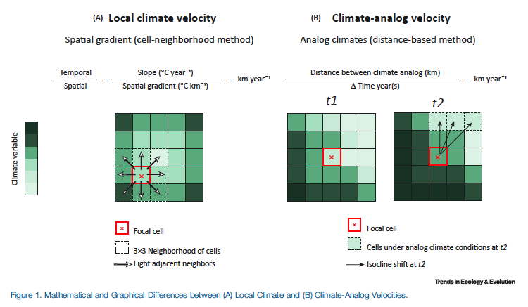
Climate velocity is a vector that describes the speed and direction that a point on a gridded map would need to move to remain static in climate space (e.g., to maintain an isoline of a given variable in a univariate environment) under climate change. From an ecological perspective, climate velocity can be conceptualized as the speed and direction in which a species would need to move to maintain its current climate conditions under climate change. For this reason, climate velocity can be considered to represent the potential exposure to climate change faced by a species if the climate moves beyond the physiological tolerance of a local population. See(Brito-Morales et al. 2018).

Install the R package: GitHub Repo

To calculate climate velocity the R package VoCC provides a comprehensive collection of functions that calculate climate velocity and related metrics from their initial formulation to the latest developments. See Garcia Molinos et al. 2019.

# Load the monthly raster object
  rs <- terra::rast("data/tos_Omon_GFDL-ESM4_ssp585_r1i1p1f1_gr_201501-203412.tif")
# Establish the time period of interest (if applicable)
  from = 2015
  to = 2034
# If Raster is monthly, get annual mean
  index <- rep(1:nlyr(rs), each = 12, length.out = nlyr(rs))
  rs <- raster::stackApply(x = raster::stack(rs), indices = index, fun = mean)

# Calculate VoCC
  # Temporal trend (slope)
    slp <- tempTrend(rs, th = 10)
  # Spatial gradient (gradient)
    grad <- spatGrad(rs, th = 0.0001, projected = FALSE)
# VoCC local gradient
  vocc <- gVoCC(slp, grad)
  vocc$voccMag[] <- ifelse(is.infinite(vocc$voccMag[]), NA, vocc$voccMag[]) # replace inf with NAs

Brito-Morales, Isaac, Jorge García Molinos, David S. Schoeman, Michael T. Burrows, Elvira S. Poloczanska, Christopher J. Brown, Simon Ferrier, et al. 2018. “Climate Velocity Can Inform Conservation in a Warming World.” Trends in Ecology & Evolution 33 (6): 441–57. https://doi.org/10.1016/j.tree.2018.03.009.

Brito-Morales, Isaac, David S. Schoeman, Jason D. Everett, Carissa J. Klein, Daniel C. Dunn, Jorge García Molinos, Michael T. Burrows, et al. 2022. “Towards Climate-Smart, Three-Dimensional Protected Areas for Biodiversity Conservation in the High Seas.” Nature Climate Change, April, 1–6. https://doi.org/10.1038/s41558-022-01323-7.

Burrows, Michael T., David S. Schoeman, Lauren B. Buckley, Pippa Moore, Elvira S. Poloczanska, Keith M. Brander, Chris Brown, et al. 2011. “The Pace of Shifting Climate in Marine and Terrestrial Ecosystems.” Science 334 (6056): 652–55. https://doi.org/10.1126/science.1210288.