source("zscripts/z_helpFX.R") # and the Help function just in case :-)8 Extracting Front Data (or any variable) for the Created Grid
Here, we’ll dive into the process of extracting front data—or any other variable—for the grid we created earlier. I’ll walk you through aligning spatial datasets, performing interpolations, and dealing with missing data to make sure your results are accurate and complete.
8.1 Data import
Source the required helper.
8.2 A helper function to replace NA with nearest neighbor values
Before proceeding, we need to define a helper function to replace NA values with the nearest neighbor’s values. This is necessary because when interpolating non-equal data, such as a raster, onto an equal-area grid, you may encounter NA values during the overlapping process. These NA values typically arise because the interpolation does not have sufficient data points in certain areas, leading to gaps in the resulting grid.
When performing spatial operations like calculating a weighted mean, R may not be able to handle these NA values correctly, which can result in inaccurate or incomplete results. By replacing NA values with the nearest neighbor’s values, we ensure that the entire grid is populated with meaningful data, allowing for accurate calculations and analyses.
replace NAs function (written by Jason Everett)
fCheckNAs <- function(df, vari) {
    if (sum(is.na(pull(df, !!sym(vari)))) > 0) { # Check if there are NAs in the specified variable

      gp <- df %>%
        mutate(isna = is.finite(!!sym(vari))) %>%
        group_by(isna) %>%
        group_split()  # Split the data frame into two groups: with and without NAs

      out_na <- gp[[1]]    # DataFrame with NAs
      out_finite <- gp[[2]] # DataFrame without NAs

      d <- st_nn(out_na, out_finite) %>% # Find the nearest neighbor for each NA value
        unlist()

      out_na <- out_na %>%
        mutate(!!sym(vari) := pull(out_finite, !!sym(vari))[d]) # Replace NAs with the nearest neighbor values

      df <- rbind(out_finite, out_na) # Combine the data frames back together
    }
    return(df)
  }
8.3 Read, Extract, and Weighted Mean Interpolation
This code is designed to process spatial data by working with a raster dataset and a shapefile that defines specific areas of interest. It aligns both the raster data and the shapefile to the same map projection. Then, it calculates the average values of the raster data within each defined area, accounting for differences in cell size. If any data points are missing, the code fills in those gaps using the nearest available data.
The code is also designed to run on multiple processor cores simultaneously, making it faster and more efficient, especially when dealing with large datasets.
Warning
This code may take some time to process. For the sake of this workshop, you can skip this step as the necessary files have already been provided in data_rout/fsle_rds.
# Define paths to the input and output directories, and the desired projection
rs_path = "data_raw/fsle_rs"  # Directory where the raw raster files are stored
shp_path = "input_layers/boundaries/PUs_NA_04km2.shp"  # Path to the shapefile representing planning units
outdir = "data_rout/"  # Directory where output files will be saved
proj.geo = "ESRI:54030"  # Projection to be used for transforming spatial data

# Get only the first .tif raster file in the specified directory as an example
rs_fsel <- list.files(path = rs_path, pattern = ".tif", full.names = TRUE) [1]

# Loop through each raster file in the list
for (j in seq_along(rs_fsel)) {

  # Step 1: Read the shapefile and transform it to the desired projection
  shp_file <- st_read(shp_path) %>%
    st_transform(crs = terra::crs(proj.geo))

  # Step 2: Read the raster file and set its CRS to EPSG:4326 (WGS 84)
  rs_file <- rast(rs_fsel[j])
  crs(rs_file) <- terra::crs("EPSG:4326")

  # Step 3: Calculate the cell size (area) of the raster and reproject both the raster and its weights to the desired CRS
  weight_rs <- terra::cellSize(rs_file)  # Calculate the cell size (area) of the raster
  rs_file <- terra::project(rs_file, y = terra::crs(proj.geo), method = "near")  # Reproject the raster
  weight_rs <- terra::project(weight_rs, y = terra::crs(proj.geo), method = "near")  # Reproject the cell size raster

  # Step 4: Rename the raster layers if there are duplicated names to avoid conflicts
  if (sum(duplicated(names(rs_file))) != 0) {
    names(rs_file) <- seq(from = as.Date(names(rs_file)[1]),
                          to = as.Date(paste0(paste0(unlist(stringr::str_split(names(rs_file)[1], "-"))[1:2], collapse = "-"), "-",length(names(rs_file)))),
                          by = "day")
  } else {
    rs_file
  }

  # Step 5: Extract raster values for each planning unit (polygon) using weighted mean
  rs_bypu <- exact_extract(rs_file,
                           shp_file,
                           "weighted_mean",
                           weights = weight_rs,
                           append_cols = TRUE,
                           full_colnames = TRUE)

  # Step 6: Join the extracted values back to the shapefile based on the FID (unique identifier)
  rs_shp <- dplyr::right_join(shp_file, rs_bypu, "FID")

  # Step 7: Clean up column names by removing the "weighted_mean." prefix
  colnames(rs_shp) <- stringr::str_remove_all(string = names(rs_shp), pattern = "weighted_mean.")

  # Step 8: Set up parallel processing for handling large data sets
  cores  <-  detectCores() -1  # Define the number of cores to use for parallel processing
  cl <- makeCluster(cores)  # Create a cluster object for parallel processing
  registerDoParallel(cl)  # Register the cluster for use in parallel processing

  # Step 9: Prepare to process each column of the data frame in parallel
  nms <- names(rs_shp)  # Get the column names
  nms <- nms[nms != "geometry" & nms != "FID"]  # Exclude geometry and FID columns from processing
  ls_df <- vector("list", length = length(nms))  # Initialize a list to store results

  # Step 10: Process each variable in parallel using foreach loop
  df1 <- foreach(i = 1:length(nms), .packages = c("terra", "dplyr", "sf", "exactextractr", "nngeo", "stringr")) %dopar% {
    single <- rs_shp %>%
      dplyr::select(FID, nms[i])  # Select the FID and the current variable
    rs_sfInt <- fCheckNAs(df = single, vari = names(single)[2]) %>%  # Apply the helper function to handle NAs
      as_tibble() %>%
      dplyr::arrange(FID) %>%
      dplyr::select(-FID, -geometry)  # Remove the FID and geometry columns
    ls_df[[i]] <- rs_sfInt  # Store the processed data in the list
  }

  # Step 11: Stop the parallel processing cluster
  stopCluster(cl)

  # Step 12: Combine all the processed data into a single data frame
  rs_sfInt <- do.call(cbind, df1) %>%
    as_tibble()

  # Step 13: Generate a filename for the output based on the raster file's name
  ns <- stringr::str_remove_all(basename(rs_fsel[j]), pattern = ".tif")

  # Step 14: Save the processed data as an RDS file in the specified output directory
  saveRDS(rs_sfInt, paste(outdir, ns, ".rds", sep = ""))
}
8.4 Plot the output
Plotting the output is straightforward. Just follow these steps in the note below:
Reading and ploting the FSLE data
1. Load and Prepare Data
pus <- st_read("input_layers/boundaries/PUs_NA_04km2.shp")
fsle <- readRDS("data_rout/fsle_rds/dt_global_allsat_madt_fsle_2016-06.rds") %>%
  dplyr::mutate(across(everything(), ~ .x * -1))
DFfsle <- cbind(pus, fsle$`2016-06-01.area`)
In this step, we load the planning unit shapefile and the FSLE data for June 2016. We also adjust the FSLE values and combine them with the shapefile data.
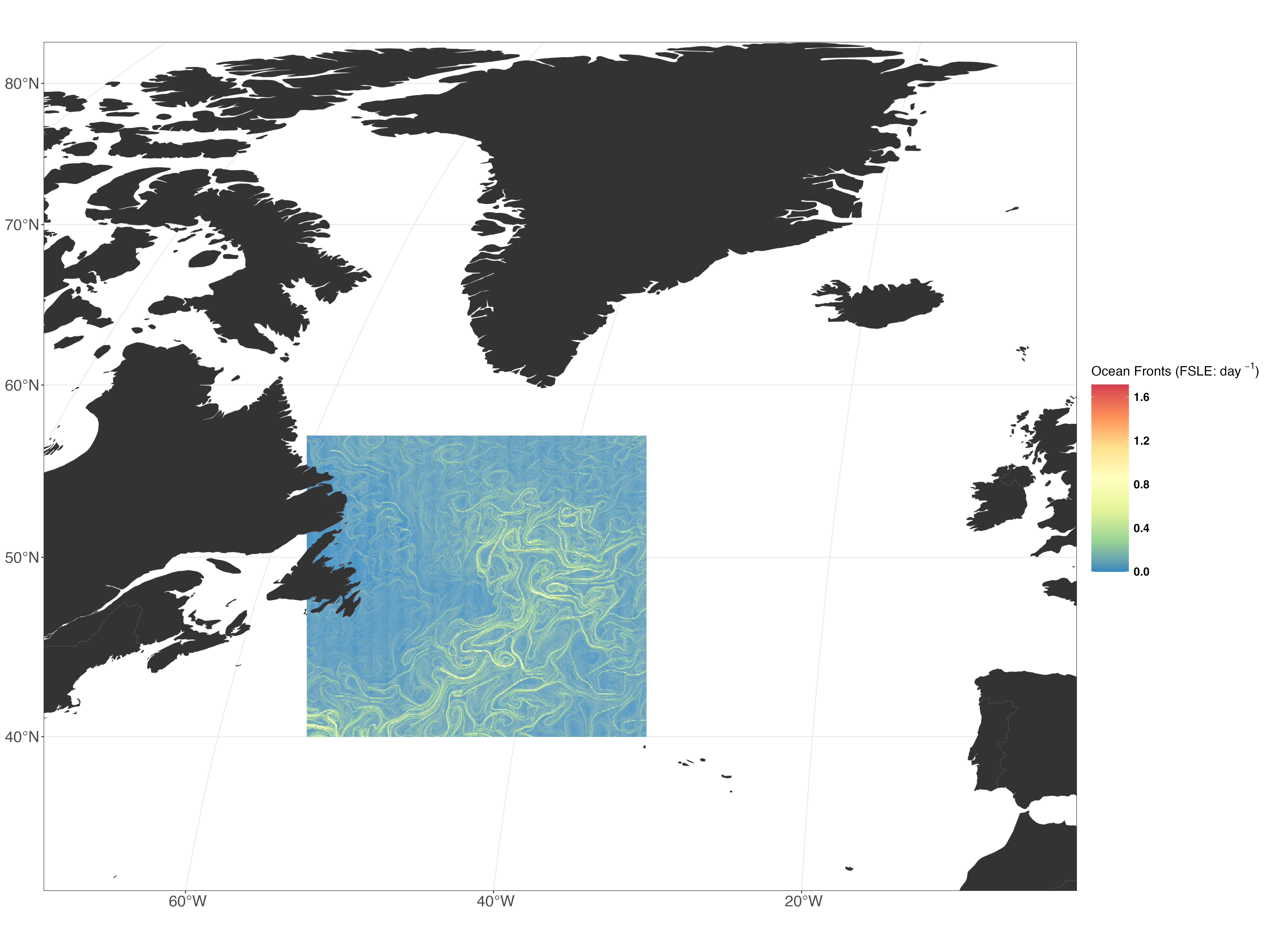
2. Create the Plot
p1 <- ggplot() +
  geom_sf(data = DFfsle, aes(fill = fsle..2016.06.01.area.), colour = NA) +
  scale_fill_distiller(palette = "Spectral",
                       direction = -1,
                       oob = scales::squish,
                       guide = guide_colourbar(title.position = "top",
                                               title = expression("Ocean Fronts (FSLE: day" * " "^{-1} * ")"))) +
  geom_sf(data = worldsf_rob, size = 0.05, fill = "grey20") +
  theme_bw() +
  coord_sf(xlim = c(st_bbox(worldsf_rob2)$xmin + 85000, st_bbox(worldsf_rob2)$xmax - 85000),
           ylim = c(st_bbox(worldsf_rob2)$ymin + 70000, st_bbox(worldsf_rob2)$ymax - 70000),
           expand = TRUE) +
  theme(plot.title = element_text(face = "plain", size = 20, hjust = 0.5),
        plot.tag = element_text(colour = "plain", face = "bold", size = 23),
        axis.title.y = element_blank(),
        axis.title.x = element_blank(),
        axis.text.x = element_text(size = rel(2), angle = 0),
        axis.text.y = element_text(size = rel(2), angle = 0),
        legend.title = element_text(colour = "black", face = "bold", size = 15),
        legend.text = element_text(colour = "black", face = "bold", size = 13),
        legend.key.height = unit(1.5, "cm"),
        legend.key.width = unit(1.5, "cm"))
Here, we create a plot using ggplot2 R package. The plot shows the FSLE data with a color scale representing ocean fronts. We also add geographic boundaries and customize the plot’s appearance.
3. Save the Plot:
ggsave("figures/dt_global_allsat_madt_fsle_2016-06.png", plot = p1, width = 20, height = 15, dpi = 350, limitsize = FALSE)Finally, we save the plot as a high-resolution PNG file, specifying the dimensions and quality settings.